CaseConnect 3.0: Spot connected cases faster

Eighteen months ago we wrote about connecting cases : the simple observation, backed by our research , that a large share of cryptoasset investigations are quietly connected to one another. 41% of cyberfraud cases and 96.9% of sextortion cases in that study shared an address, a cluster, or a collector wallet with at least one other case. Investigators were working the same perpetrators in parallel, often without knowing it.

CaseConnect was our answer: a tool that surfaces those connections so agencies can pool what they know instead of duplicating effort. Since then, more agencies have added more cases, and the connection network has grown with them. That growth also taught us something about the interface itself: the original, graph-first way of exploring case connections was visually appealing, but it wasn’t always the most efficient route to an answer.

So we redesigned it. CaseConnect 3.0 doesn’t throw away the graphical representation (it’s still there), but it shifts it into the background and builds the interface around the use cases we actually see in the field: quickly finding the connections for the cases that matter, and stepping back to see the bigger trends in the data, such as how cases and connected cases have grown over time, which is a clear signal of how well the approach is working. In this blog post we walk you through the new interface: how to create cases and how to inspect case connections.

The approach has since moved from study to daily practice. Today CaseConnect holds around 1,700 active cases from 13 participating agencies, with more than 4,200 connections between them: 44% of the cases connect to at least one other case.

Why connections still matter

The premise hasn’t changed, but the case load has. Cryptoasset-related crime keeps generating more investigations than any single unit can work in isolation, and the value of a connection compounds as the network grows: every case you add is checked against every case already there. A match can mean a shared suspect, a shared cash-out point, or a shared piece of infrastructure, and it can cross crime areas, jurisdictions, and borders.

CaseConnect looks for those matches on three levels, the same heuristics our research validated:

• Common addresses: two cases that reference the exact same cryptoasset address.
• Common clusters: addresses that GraphSense’s clustering heuristics assign to the same cluster (the same likely real-world actor), even when the addresses themselves differ.
• Common collectors: wallets that aggregate funds from multiple cases, one hop downstream from the perpetrator wallets where the money pools.

What 3.0 changes is not what gets connected, but how clearly you can see it.

What’s new in 3.0

We start with the interface, because that is where the redesign is most visible. In CaseConnect 2.0 all the data was already there, but the interface wasn’t tailored to the most important use cases. Its graphical view was nice to look at, yet it wasn’t an efficient way to find the right data points. 3.0 keeps the data and reorganizes the interface around the three things you actually want to do: add a case, understand a single case’s connections, and survey all of your cases at once, with a redesigned UI that makes each of them direct.

Beyond optimizing the user flows and how data is presented, we also worked on the responsiveness of the interface, and a big part of that happens out of sight. The connection-finding now runs as server-side precomputation: instead of computing matches on demand while you wait, the connections are calculated and kept up to date in the background. So by the time you open a case, the work is already done, and there’s no spinner while the tool figures out what connects to what. The practical effect is a noticeably smoother experience: the interface is faster, the connection results stay complete and up to date, and newly added cases are reconciled against the existing network quickly rather than on a slow ad-hoc pass.

And because data is the whole point of the tool, adding it is now front and center, including importing many addresses at once instead of entering them one by one.

Adding a case

Adding a case is the first thing most users do, so it’s the first thing we streamlined. There are two ways to do it, depending on where you are.

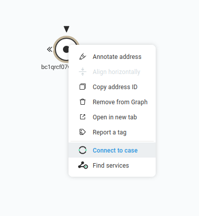
The first is straight from Pathfinder , our investigation UI. While you’re working in the graph, select an address, right-click it, and choose Connect to case. This is the quick path for when you’re already tracing and spot an address that belongs to a case: you add it to a new or existing case without leaving Pathfinder.

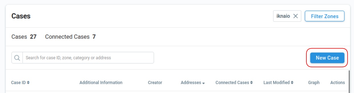
The second is from the CaseConnect overview, using the New case button in the top right. This is the path to use when you’re starting from a list rather than from the graph, and it’s where bulk import lives.

Bulk import is the important upgrade here. Investigations rarely start with a single address; you usually arrive with a list pulled from a report, a spreadsheet, or another tool. Instead of entering addresses one at a time, you can simply paste them all into a text box, and CaseConnect parses the addresses out of whatever you pasted, validates that they actually exist, and tags them to the case together.

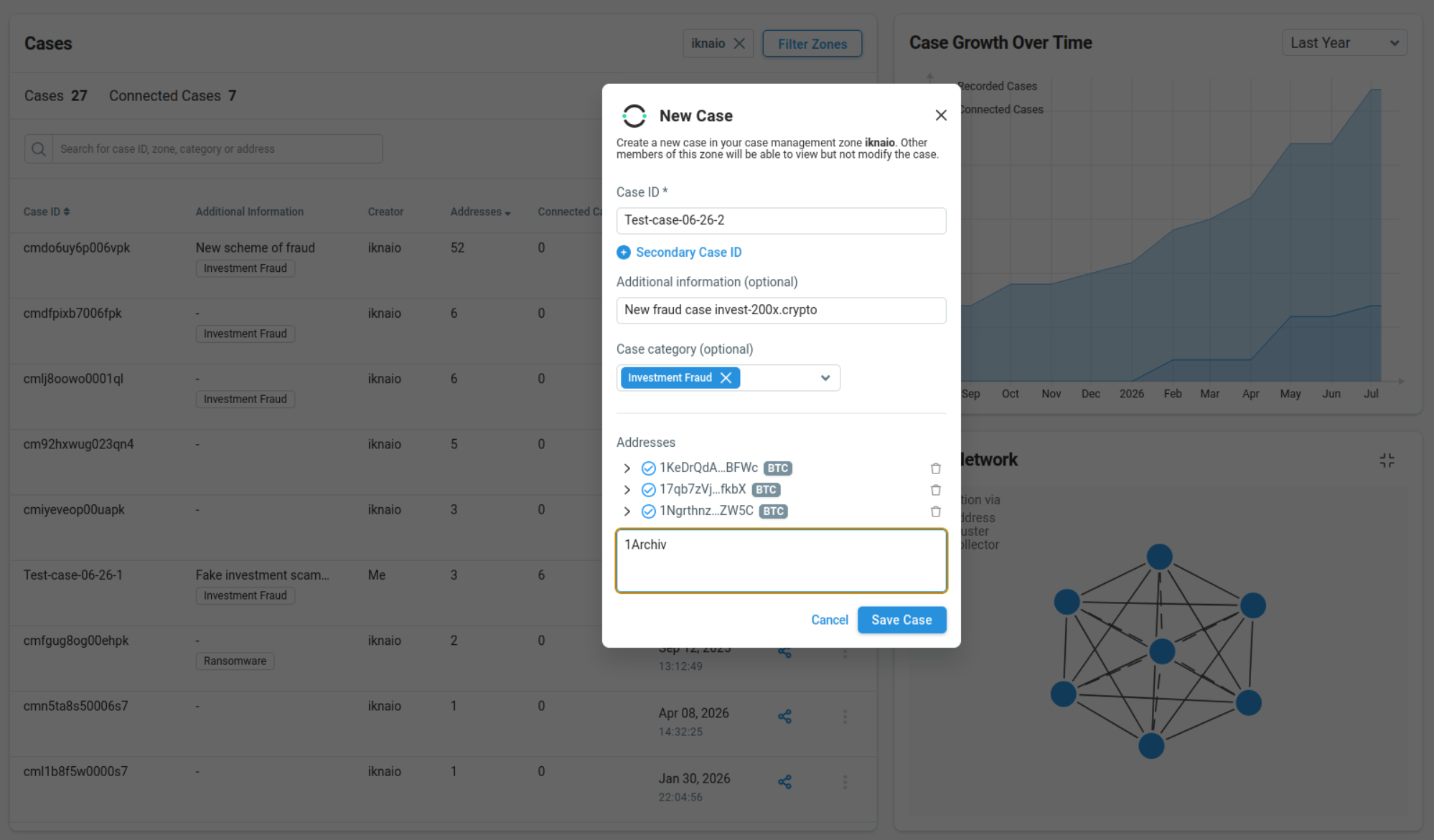
As soon as the addresses are in, CaseConnect checks them against everything already in your visible zones. You don’t run a separate “find connections” step; adding the data is the query.

Seeing a case’s connections

Once a case has addresses, the interface shows you what it connects to. This is where the rehaul is most visible: connections are now presented in tabular form first and foremost, a clear, scannable list of the cases yours connects to and why. The visual network representation from CaseConnect 2.0 is still there, but it now sits in the background rather than being the first thing you see. It has also been improved while it was at it: where CaseConnect 2.0 spread the heuristics across a separate network per type, the new network view brings all connection types together in a single graph, so when you do want the visual, it’s the whole picture in one place.

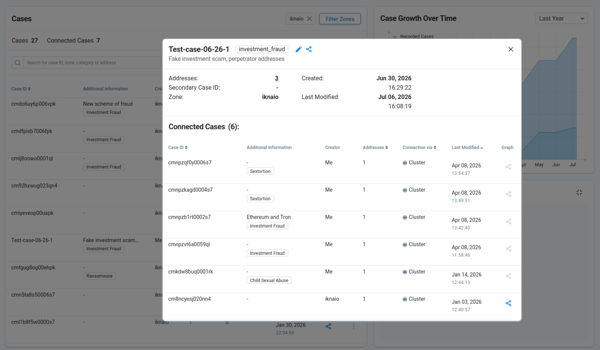
The connected-cases table lists every case that links to the one you’ve selected, and crucially a connection via column spells out the reason for each one: a common address, a common cluster, or a common collector. This is the part that used to be hard. In CaseConnect 2.0, seeing why two cases connected meant looking across separate network views, one per heuristic, and reading it off the graph. Now it’s a single column in a single list. The connection type shown there also carries the strength of the signal, since a shared address is more direct than a shared collector, and having it spelled out means you can scan and sort by it instead of inferring it.

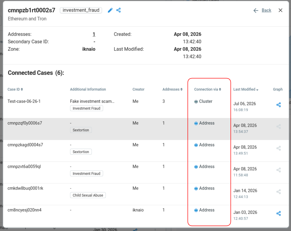
From there you can follow a connection through to the connected case, within the limits of your zone permissions. On that case you see its details: the other addresses linked to it, and its internal case ID, which (depending on the institution) typically tells you which group to contact. You can also keep going transitively, following that case’s own connections one step further out to see what it links to. And if a Pathfinder graph was attached to the case, a blue graph icon opens it, giving you the full investigative context behind the case and showing where the work potentially overlaps with yours.

The bigger picture

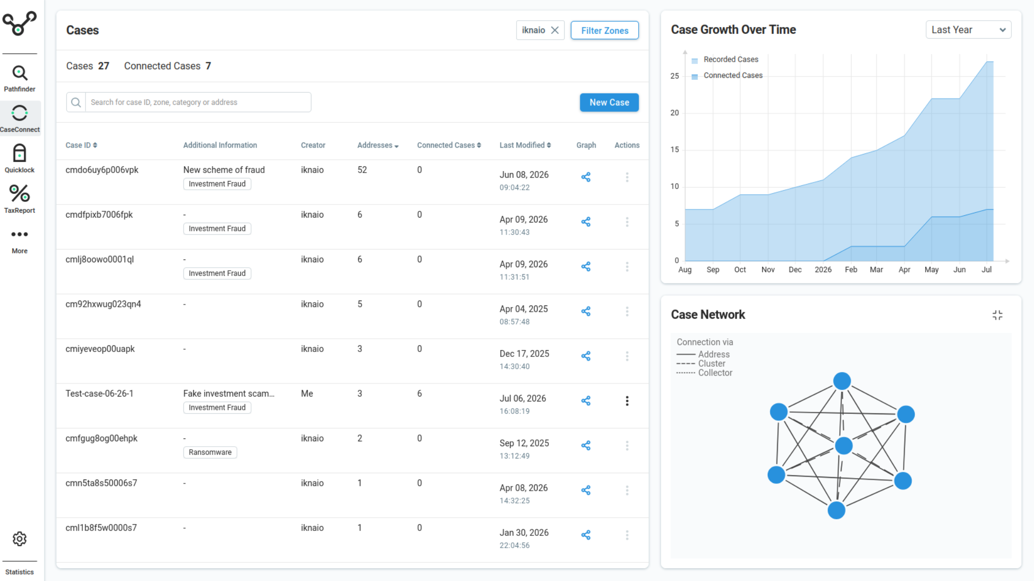
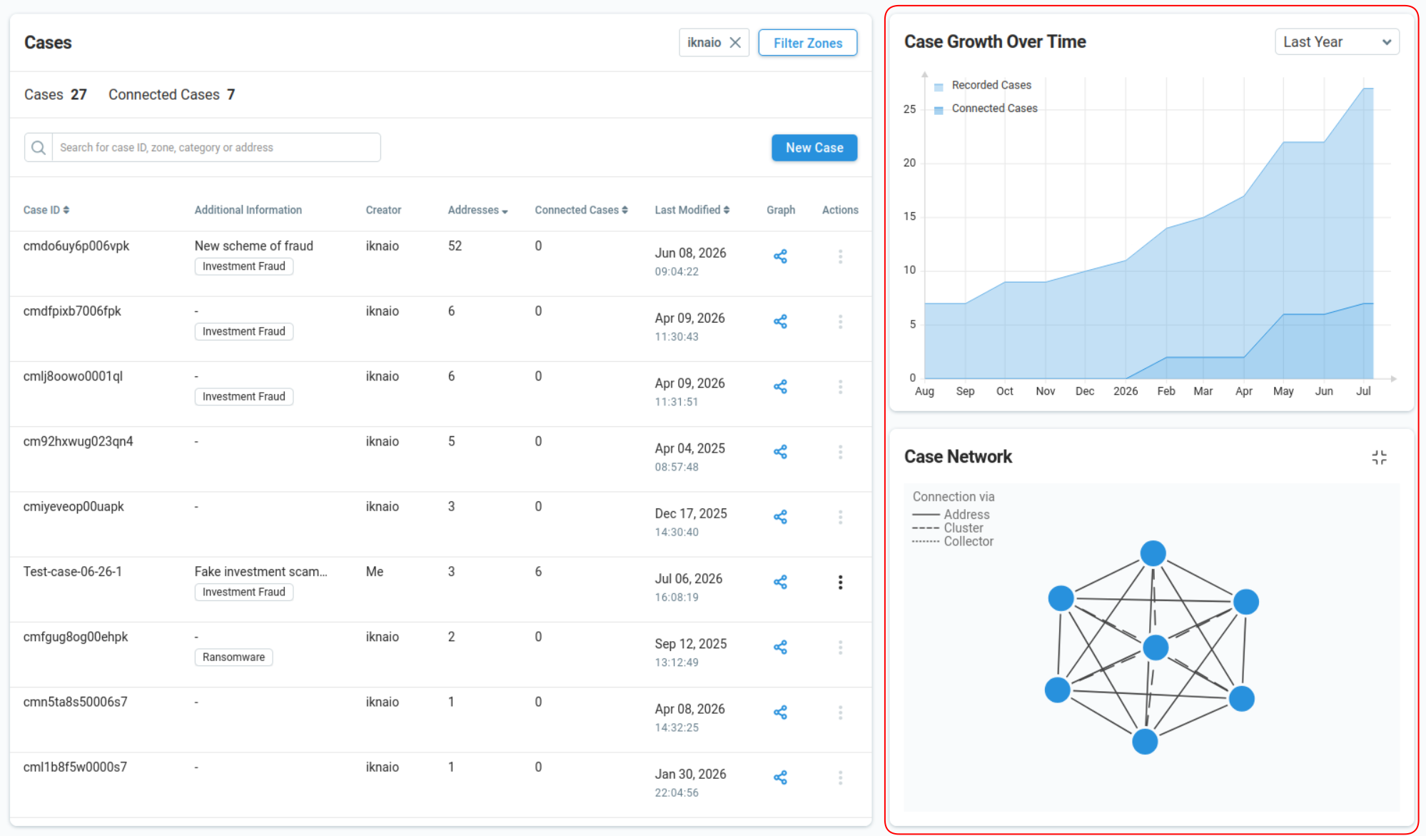
Looking at one case at a time is the investigator’s view. The overview is the cases list: all of your cases in one place, with the connected ones called out. For a supervisor, the case network and the case growth over time are what turn that list into context, showing at a glance how the cases group together, where the work overlaps, and how the whole picture is developing.

Instead of opening cases individually to discover that two of them overlap, the overview is the single place where all of your cases live. You can sort it by number of connections, by the number of addresses attached to a case, or by when it was last modified, and search across every case by ID, name, category, and more. Sorting by number of connections brings the most-connected cases, the ones where the same actors keep showing up, to the top, which is exactly the prioritization signal the original research argued for: rather than treating cases as a flat queue, you can work the most connected ones first. Opening a case from here gives you the same details and attached-graph view described above, and you can filter by zone, choosing which zones contribute to the connections you see, to widen the view to the full shared network or narrow it to your own.

Watching the network grow

The last addition is one we’re especially happy with, because it makes the core idea of CaseConnect visible. The interface now charts how the number of cases and the number of connected cases have grown over time.

Every case an agency adds is checked against the cases it can actually see, which is governed by zone visibility: CaseConnect doesn’t automatically check against the entire database, and it’s up to the participants to make their cases visible to one another. Within that shared scope, the share of cases that connect to at least one other case tends to climb as the network grows, since each case you add has more existing cases to match against. Seeing the two curves side by side, the total number of cases and the number of connected cases, makes the network effect concrete: the tool gets more useful the more it’s used, and the growth chart is the proof.

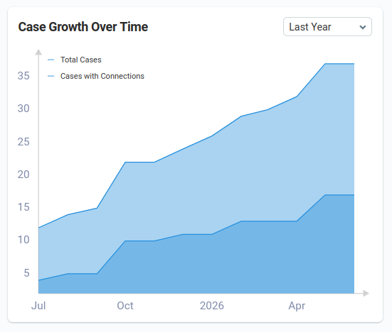
It also gives the participants a powerful way to communicate the vision and bring more people on board: the growth curves are concrete proof that the more cases everyone contributes, the more of everyone’s cases end up connected. That makes them an easy argument for getting the next agency to join.

Conclusion

CaseConnect 3.0 keeps the heuristics that the research proved out and rebuilds everything around them. Adding cases is faster, especially with bulk address import. Seeing why two cases connect is now easy: a single list with a connection-type column, where before you had to read it off separate network views, one per heuristic. The overview turns a pile of cases into a map of which ones are connected, and the growth view shows that map filling in over time. With server-side precomputation underneath, all of it is quicker and always up to date.

The goal is the same as it was eighteen months ago, to help investigators find the connections between their cases and stop duplicating each other’s work, but 3.0 helps you do it better and faster.

If you’d like to see CaseConnect 3.0 on your own cases, or learn how the zone model lets you share connections without sharing case detail, get in touch .